
What is Pivot Table in Excel and Why is it Useful?
Pivot tables are one of the most powerful and useful features in Excel. With very little effort, you can use a pivot table to build good-looking reports for large data sets.
You can think of a pivot table as a report. However, unlike a static report, a pivot table in excel provides an interactive view of your data. With very little effort (and no formulas) you can look at the same data from many different perspectives. You can group data into categories, break down data into years and months, filter data to include or exclude categories, and even build charts.
The beauty of pivot tables in excel is they allow you to interactively explore your data in different ways. Therefore, it helps to make data analysis easier and more effective.
5 Ground Rules before Creating Pivot Table in Excel
Before we move on to learn how to create a Pivot Table in Excel, it is important to understand the 5 ground rules when using the pivot table feature in Excel:
- Datasets must be organized in rows with each row representing a record
- Datasets must have a unique column header that identifies the column field
- There should be NO blank rows and blank columns
- All empty cells should contain zero or text (e.g. nil)
- There should be no merge cells in the datasets

Image: Sample of Datasets for Pivot Table in Excel
In summary, it is best to use your raw data report (as shown in the image above) to create your pivot tables for data analysis. If you have an existing data report that has already been summarised (with total, subtotals, or average value), it will hinder the ability of the pivot table in Excel to produce different slices of the data. Therefore, you will need to remove it for better analysis with pivot table in Excel.
If you want to advance your current level of Excel skills and be more qualified in working with pivot tables in excel, then don’t miss out on our 1-Day Pivot Table for Microsoft Excel: Basic to Intermediate Workshop. For those who have good working knowledge on Pivot Table and would like to advance further, you may consider our Advanced Pivot Table for Microsoft Excel course.
Below are 3 simple yet useful features to start your pivot table journey
Building a Pivot Table in Excel in Just One Minute
Many people think building a pivot table in excel is complicated and time-consuming, but it’s simply not true. Compared to the time it would take you to build an equivalent report manually, pivot tables are incredibly fast. If you have well-structured source data, you can create a pivot table in less than a minute. Start by selecting any cell in the source data.
Next, follow these four steps:
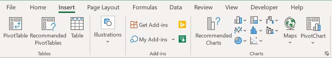
1. On the Insert tab of the ribbon, click the PivotTable button
2. In the Create PivotTable dialog box, select the data range and click OK

3. Drag a “label” field into the Row Labels area (e.g. product name)
4. Drag a numeric field into the Values area (e.g. revenue)
Voila ~ in just a minute, you got your first pivot table in excel. Well done!

The pivot table above shows total revenue by product, but you can easily rearrange fields to show total revenue by customer, by product line, by month, and so on by dragging different fields to the Rows or Values area.
Show Totals as a Percentage
In some of the cases, you’ll want to show a percentage rather than a count in your pivot table. For example, perhaps you want to show a breakdown of revenue by product. But, rather than show the total revenue for each product, you want to show revenue as a percentage of the total revenue. You can do so by performing this one simple step (assuming you have created the pivot table):
1. Right-click the Revenue field, and set “Show Values As” to “% of Grand Total”
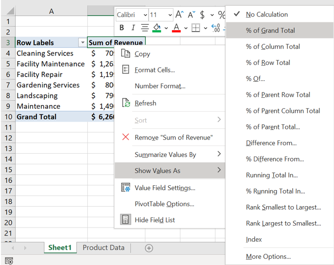
Voila ~~ your total revenue is now shown as a total percentage.
Drill Down to See (or Extract) the Data behind any Total
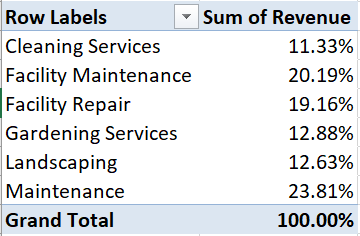
Whenever you see a total displayed in a pivot table, you can easily see and extract the data that makes up the total by “drilling down”. For example, assume you are looking at a pivot table that shows total revenue by product name. You can see that the product name “Cleaning Services” constitute a total revenue of 11.33%, but you want to see the list of customers who purchased this product. To see the list of records that make up this number/percentage, double-click directly on the number 11.33% and Excel will add a new sheet to your workbook that contains the exact data used to calculate 11.33% revenue as shown below.

If you are not getting enough tips from the above, watch the following 1.5 hours webinar facilitated by Ms. Valene Ang on how to create Pivot Table in Excel:
Get Personalised Coaching on Pivot Table in Excel at Aventis

Pivot Table for Microsoft Excel: Basic to Intermediate Workshop is one of the best-selling excel courses at Aventis, which will give you a very comprehensive guide to start your data exploration and analysis with pivot table in Excel. If you are keen to mastering pivot table in Excel, simply click here to register to join our course. Not sure if this is the right course for you? Get in touch with us at 6720 3333 or email training.aventis@gmail.com and we are happy to recommend the most suitable Microsoft Excel courses for you!
Bonus: Useful Shortcuts for Pivot Table in Excel
| Alt + N + V | Open Pivot Table Wizard |
| Alt + F1 | Create Pivot Chart on Same Worksheet |
| F11 | Create Pivot Chart on New Worksheet |
| Alt + Shift + ArrowRight | Group Pivot Table Items |
| Alt + Shift + ArrowDown | Ungroup Pivot Table Items |
Sources: